Yield per Acre in Agriculture: Precision Farming’s Revenue Impact KPI in 2027

Two competing ways to run the metric: maximize yield or maximize margin

Every operation that installs precision hardware eventually confronts the same fork, and most people never name it out loud. There are two coherent strategies you can run against yield per acre, they point at different agronomic decisions, and running both at once is how farms end up with a spreadsheet full of impressive numbers and a bank line that keeps growing.

Option A — the yield-maximization play. You treat yield per acre as the number to push, and you spend inputs until the last incremental unit stops paying. In practice that means seeding rates at or above the agronomic optimum in your best zones, full-rate nitrogen with in-season top-dress, fungicide passes on the calendar rather than on threshold, and irrigation scheduled toward the wet side of the crop's water requirement. The measurement discipline is straightforward: yield monitor data by zone, calibrated against scale tickets, compared against a county or state benchmark. The narrative is easy to sell to a lender, easy to explain to a landlord, and easy to compare to a neighbor over coffee. In a high-price year with cooperative weather, this play prints money — an extra 15 bushels of corn at $5 is $75 per acre of pure top line, and if the incremental input cost was $30, you cleared $45.

Option B — the cost-optimization play. You hold yield roughly flat and attack the input side, using the same precision data to find where you have been over-applying. Variable-rate nitrogen prescriptions typically cut total nitrogen 10–20% on fields with meaningful soil variability, because the low-organic-matter sand streaks and the eroded hilltops were never going to convert the full rate into grain. Variable-rate seeding pulls population down in the weak zones and pushes it up in the strong ones, often at a net-neutral seed cost. Variable-rate irrigation on a pivot skips the sand blowouts and the field roads. The yield number barely moves — sometimes it drops a bushel or two — but the cost per bushel falls, and cost per bushel is the number that determines whether you survive a $3.80 corn market.

The tension is real and it is not resolvable by picking the "better" one. Option A wins when commodity prices are high relative to input prices and when your ground has low variability — uniform, high-quality soil rewards uniform, high inputs. Option B wins when the price ratio inverts, when your fields have high internal variability, and when you have working capital constraints that make a $500-per-acre input bill genuinely risky. Most farms sit somewhere in between and should be explicit about where.

There is a third position worth naming because people fall into it accidentally: the uniformity play, which targets the yield variability index rather than the mean. Here the goal is to compress the spread between your best and worst zones, on the theory that the bottom quintile of acres is where the money leaks. This is neither pure yield nor pure cost — it is a reallocation strategy, and it often produces the best three-year return because fixing a 140-bushel zone to 180 is easier than pushing a 240-bushel zone to 250. Diminishing returns are steep at the top of the yield curve and shallow at the bottom.

What makes 2027 different from 2017 is that the data cost of running any of these has collapsed while the input cost of running Option A has not. Yield monitors ship standard on new combines. Satellite imagery at field resolution is effectively a commodity. Soil electrical conductivity mapping and grid sampling remain the genuine expense, and they are the thing most operations underbuy. You cannot run a credible variable-rate prescription off imagery alone — imagery tells you where the crop is struggling this season, soil data tells you why, and only the second one lets you write a prescription for next season.

A practical framing: yield per acre is your revenue metric, cost per bushel is your resilience metric, and profit per acre is the scoreboard. If you only instrument one, instrument profit per acre by zone. If you can instrument two, add cost per bushel. Yield per acre alone is the metric that has bankrupted the most farms, because it is the one that feels like progress while the margin compresses underneath it.

How to decide which play your ground actually rewards

The decision is mechanical if you have the data. Run it in this order and stop at the first fork that gives you a clear answer.

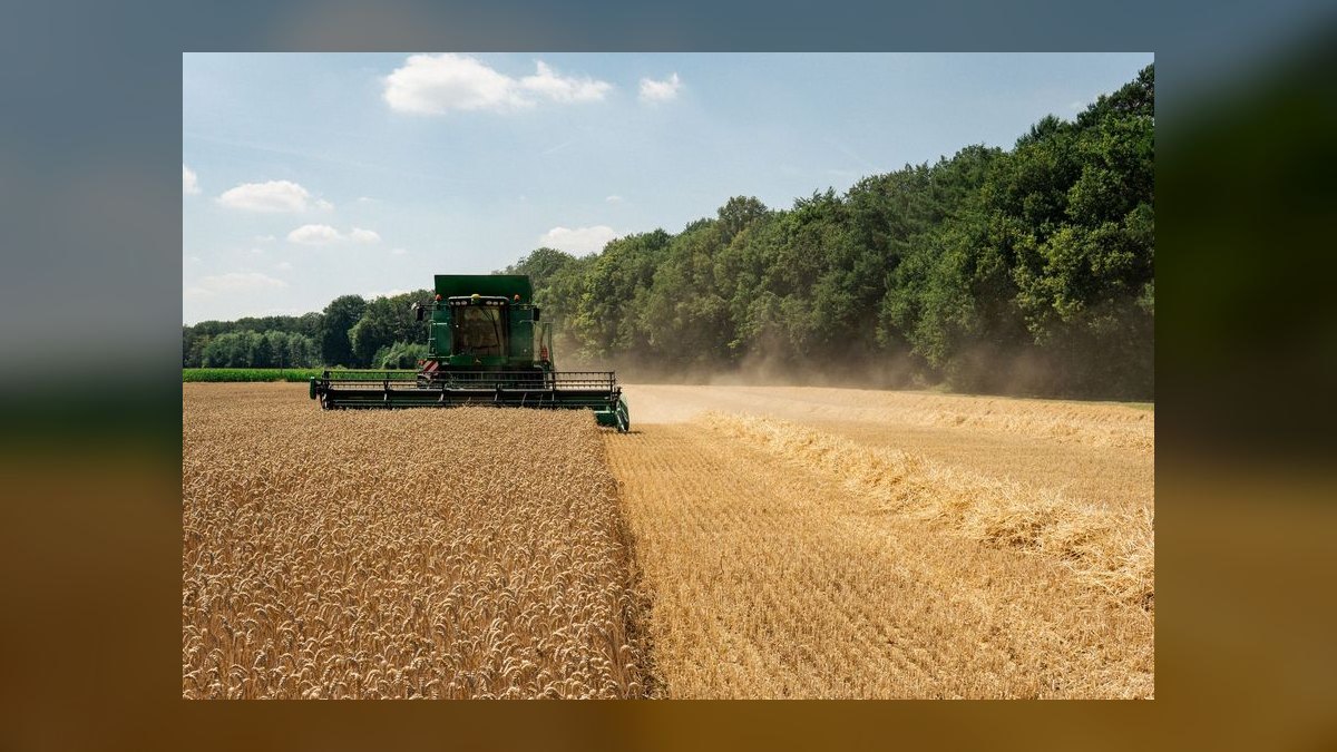
Step one: measure your internal variability before you measure anything else. Pull three to five years of calibrated yield monitor data, clean it for the obvious artifacts — start and stop passes, grain flow lag, partial swaths, headland turns — and compute the coefficient of variation across zones within each field. This is standard deviation of zone yields divided by mean zone yield, expressed as a percentage. A field under roughly 10–12% CV is functionally uniform; variable-rate work will produce marginal returns because there is little to vary against. A field above 25% CV has a real spatial problem and is the highest-return target on the farm. Most Midwestern row-crop fields land between 15% and 25%.

Step two: check whether the variability is fixable or structural. This is where operations go wrong. Some variability responds to management — pH that drifted, phosphorus and potassium drawn down in the historically high-yielding areas, compaction from a wet harvest, drainage that needs tile. Some is structural: shallow topsoil over gravel, a sand ridge, a saline seep, a north-facing slope that stays cold. Fixable variability justifies Option B or the uniformity play, because you are buying a yield response. Structural variability justifies a different move entirely — stop spending full inputs on ground that cannot convert them, and accept the lower yield on those acres while banking the input savings. Some operations go further and take chronically unproductive acres out of production into a conservation program, which is a legitimate profit-per-acre decision even though it looks terrible as a yield-per-acre decision.

Step three: run the price ratio. Compute the break-even yield response for the input you are considering adding. For nitrogen: divide the price per pound of nitrogen by the price per bushel of corn to get the pounds of nitrogen you must convert into one bushel to break even. At $0.50/lb nitrogen and $4.50 corn, the ratio is about 0.11 — you need roughly nine additional bushels per hundred pounds of nitrogen to justify the pass. At $0.80/lb nitrogen and $3.90 corn, the ratio nearly doubles and the same agronomic response no longer pays. This single calculation flips more farms from Option A to Option B than any agronomic argument ever will, and it needs to be re-run every season because both terms move.

Step four: check your working capital position. A farm with a fully drawn operating line and no cushion should not run Option A regardless of what the agronomy says, because Option A concentrates risk. You are spending more per acre up front against a yield that weather can erase. Option B lowers the per-acre bet. This is a financial decision that presents as an agronomic one.

The numbers behind each play

Concrete figures matter more than the framework, so here is what each path actually looks like on a thousand-acre corn operation. Treat every number as a planning range you must replace with your own records — input prices, cash rent, and basis vary enormously by region and year.

Baseline. U.S. average corn yield has run in the 170–180 bushel-per-acre range in recent years, per USDA NASS annual crop production summaries. Variable costs for corn — seed, fertilizer, crop protection, drying, and fuel — commonly land in the $400–$600 per acre band, with fertilizer alone swinging that range by $100 or more depending on nitrogen prices. Cash rent in productive Corn Belt counties frequently sits between $200 and $300 per acre and is often the single largest line item. At 180 bushels and $4.50 corn, gross revenue is $810 per acre. Subtract $500 variable and $250 rent and you are at $60 per acre — which is why so many operations are one bad year from trouble.

Option A math. Suppose intensive management buys a genuine 12 bushel-per-acre lift — plausible at the top of the published 5–15% precision-farming range on responsive ground. At $4.50, that is $54 of new revenue per acre. The inputs that bought it — a higher seeding rate, a split nitrogen application with in-season top-dress, and a fungicide pass — realistically cost $30–$45 per acre together. Net gain: roughly $10–$25 per acre, or $10,000–$25,000 across the thousand acres. That is real, but notice how thin the margin is and how completely it depends on the yield response materializing. A dry August erases it. If corn is $3.90 instead of $4.50, the same 12-bushel lift grosses $47 and the play is close to break-even before you have accounted for a single hour of extra labor.

Option B math. Now suppose you leave yield flat at 180 and cut nitrogen 15% via a variable-rate prescription built on soil sampling and multi-year yield layers. On a 200 lb/acre program at $0.50/lb, that is $150 of nitrogen, and a 15% cut saves $22.50 per acre. Add a variable-rate seeding program that reallocates rather than reduces population — often close to cost-neutral on seed but worth a few bushels in the weak zones by reducing intra-row competition under stress. Add variable-rate irrigation on pivot ground, where skipping non-productive areas commonly trims water and pumping cost by 10–15%. Total savings in the $25–$40 per acre range, with far less weather exposure than Option A because you are banking a cost reduction on day one rather than betting on a harvest-time yield.

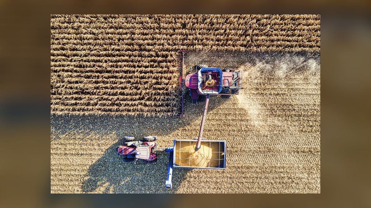
Uniformity play math. This one is often the largest number and the slowest. Say 15% of your acres — 150 acres — chronically run 40 bushels below farm average because of pH drift, phosphorus drawdown, and compaction. Correcting them is not free: variable-rate lime, a corrective phosphorus and potassium application, and possibly deep tillage or tile. Grid soil sampling at one-to-two-and-a-half-acre resolution is the enabling spend and typically runs in the $10–$25 per acre range depending on grid density and lab package, amortized over three to four years since you do not re-sample annually. If you recover 25 of those 40 bushels over two seasons, that is 150 acres × 25 bu × $4.50 = $16,875 of new revenue on a corrective spend that might total $15,000–$20,000 — payback inside two years, and the improvement persists, which neither Option A nor Option B can claim.

Technology cost, honestly. The hardware and subscription layer is smaller than people expect and the data-collection layer is larger. Yield monitoring and basic guidance are standard equipment on late-model combines and tractors. Variable-rate drive kits and section control retrofits for older implements are a per-implement capital cost in the low thousands. Farm management software subscriptions are typically annual and priced per farm or per acre. Satellite imagery services are commonly priced per acre per year. Against that, the recurring costs that actually move outcomes are soil sampling, agronomic advisory time, and the labor to calibrate and clean data — and those are the lines that get cut first when budgets tighten, which is exactly backwards.

The calibration number that hides in all of this. A yield monitor that is off by 2% misstates a 180-bushel field by 3.6 bushels per acre. Across a thousand acres at $4.50, that is roughly $16,000 of phantom or missing revenue in your records. It does not change what you actually harvested — the scale ticket is the truth — but it corrupts every zone map, every prescription, and every ROI calculation downstream. Calibrate at the start of each crop and each moisture condition, and reconcile monitor totals to scale tickets before you trust a single map.

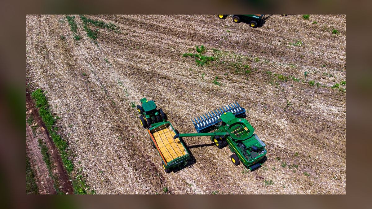
The metric to publish internally. Cost per bushel. At 180 bu/acre with $500 variable plus $250 fixed, you are at roughly $4.17 per bushel. At 220 bu/acre with $540 variable plus the same $250 fixed, you are at $3.59. That 58-cent gap is the entire margin of safety in a down market, and it is a single number a farm manager, a landlord, and a lender all understand immediately.

Building it: sequencing the first three seasons

Precision Farming programs fail on sequencing more than on technology. The common error is buying the variable-rate hardware first and the soil data last, which produces expensive prescriptions written against nothing. Reverse it.

Pre-season one — establish truth. Export every yield file you have, ideally three or more seasons. Clean it: drop the first and last twenty to thirty feet of each pass, remove partial-width swaths, correct for grain flow delay, and cut speed outliers. Uncleaned yield data routinely contains 10–20% garbage points, and those points cluster at headlands and field entries, which biases exactly the zones you care about. Reconcile each field's monitor total against scale tickets or elevator settlement sheets and record the correction factor. Then normalize each year to that year's field mean so you can stack seasons across different weather and different crops.

Season one — sample and map. Grid or zone soil sampling is the enabling spend. Grid sampling on a one-to-two-and-a-half-acre grid gives you defensible pH, phosphorus, potassium, and organic matter layers. Zone sampling — using soil survey data, electrical conductivity, elevation, and multi-year normalized yield to draw management zones, then sampling composite cores within each zone — costs less and works well where the variability is patterned rather than random. Either way you now have a *why* layer under your *what* layer. Overlay elevation and, if available, an EC map. Draw three to five management zones per field. Resist the urge to draw twenty; you cannot manage what you cannot execute with a floater and a planter.

Season one — write one prescription and hold a check strip. Do not convert the whole farm. Pick two or three fields, write the variable-rate nitrogen or seeding prescription, and leave a replicated flat-rate check strip running the length of the field through multiple zones. The check strip is the entire experiment. Without it you will have a yield map and no idea whether the prescription caused anything. Run the strips in the same direction as harvest so the combine gives you clean comparative data.

Post-harvest season one — measure the response, not the yield. Compare prescription areas to check strips within the same zone, not field averages against each other. Compute the response in bushels per acre per zone, multiply by price, subtract the input differential, and you have a per-zone return on the prescription. You will typically find the prescription paid handsomely in some zones and did nothing in others. That distribution is the finding — it tells you where to expand and where to stop.

Season two — expand where it paid, fix what is fixable. Roll the prescriptions across the fields and zones that responded. Simultaneously, start the corrective work: variable-rate lime where pH is out of range, build-up phosphorus and potassium where soil tests are below critical levels, address compaction and drainage where the yield maps and the soil pits agree. This is slow, unglamorous, and where the durable gains live.

Season two — instrument profit, not just yield. Push input costs down to the zone level. This means recording as-applied maps, not planned maps — what the machine actually put out, which differs from the prescription whenever a section control glitched or a product ran out. With as-applied cost by zone and calibrated yield by zone, you can finally compute profit per acre by zone, and that map will look meaningfully different from your yield map. Some of your highest-yielding zones are your least profitable because you spent the most there.

Season three — set policy and re-baseline. Recompute the coefficient of variation per field and compare to your season-one baseline. If CV dropped and mean yield held or rose, the uniformity play worked. Decide, per field, which of the two options that field is on going forward — and write it down, because the failure mode is drift, where a farm nominally runs variable-rate everything but has quietly reverted to flat-rate decision-making at the retailer counter. Re-sample soils on the three-to-four-year cycle. Re-run the price ratio every winter before booking inputs.

Reporting cadence that survives contact with a busy season. Weekly during harvest: calibrated yield by field and zone, moisture, and any monitor anomalies. Monthly in-season: imagery-derived crop vigor against the zone map, plus input spend to date against plan. Post-harvest: revenue per acre, cost per bushel, profit per acre, and CV by field. Annually: three-year rolling profit per acre by zone, the technology payback calculation, and the go/no-go on next year's capital.

Governance details people skip. Keep an audit trail. Yield records support crop insurance actual production history and USDA program calculations, and reconstructing them after the fact from a corrupted monitor card is miserable. Export and back up yield files off the machine at the end of each field, not at the end of harvest. Know who owns your data under each platform's terms before you upload five years of it. And keep one human-readable summary per field per year — a page that a new agronomist or a lender can read without logging into anything.

Related questions

Does a higher yield per acre always mean higher profit per acre?

No. Yield and profit decouple whenever the input cost of the last increment exceeds its revenue. A 220-bushel field carrying $600 of variable cost can be less profitable than a 185-bushel field at $440. Always pair yield per acre with cost per bushel.

How many seasons of yield data do you need before writing prescriptions?

Three minimum, five preferred. Single-season maps mostly record that season's weather. Stacking normalized years separates persistent spatial patterns — soil depth, drainage, pH — from one-off events like a hail strip or a planter skip, and only persistent patterns justify a prescription.

Can satellite imagery replace soil sampling?

No. Imagery shows where the crop is underperforming this season; soil sampling explains why. Imagery is excellent for in-season scouting, zone boundary refinement, and change detection, but it cannot report pH, phosphorus, potassium, or cation exchange capacity — the inputs a prescription actually needs.

What is a good coefficient of variation for yield across a field?

Under roughly 10–12% is uniform and offers little variable-rate upside. 15–25% is typical and is where most of the return sits. Above 25% signals a diagnosable problem — pH, drainage, compaction, or structural soil limitation — worth investigating before adding inputs.

Why does yield monitor calibration matter so much?

Because every downstream map inherits the error. A 2% calibration drift on a 180-bushel field misstates yield by 3.6 bushels per acre, which propagates into zone boundaries, prescriptions, and ROI math. The scale ticket is truth; reconcile to it every season and every crop.

FAQ

How is yield per acre actually calculated?

Total harvested weight divided by the crop's standard test weight per bushel, divided by planted acres — for corn, weight in pounds divided by 56, then divided by acres. Adjust to a standard moisture basis, typically 15.5% for corn, so seasons and fields are comparable. For precision work, run the same calculation at the management-zone level rather than the whole-field level, because a farm-wide average conceals the 20–30% internal spread that variable-rate management exists to address.

How much yield lift can precision farming realistically deliver?

Published ranges cluster around 5–15%, but the honest answer is that the lift depends almost entirely on how variable your ground is. Uniform, high-organic-matter fields have little to gain from varying rates because there is nothing to vary against. Highly variable fields with correctable problems can see much larger gains in their worst zones and none in their best. Never accept a vendor's average as your forecast; run check strips and measure your own response.

Should I start with variable-rate seeding or variable-rate nitrogen?

Nitrogen, in most corn systems. Nitrogen is a bigger dollar line, it has a steeper and more spatially variable response curve, and reducing it in low-productivity zones carries little yield risk. Variable-rate seeding is worth doing but tends to be closer to cost-neutral, functioning as a reallocation rather than a reduction. Whichever you start with, start on two or three fields with check strips, not farm-wide.

What is the single most common measurement mistake?

Reporting one farm-wide yield number. It averages away exactly the spatial signal that precision Agriculture is built to exploit, and it makes a farm look healthy while a fifth of its acres quietly lose money. The second most common is trusting an uncalibrated monitor. The third is comparing prescription fields against non-prescription fields instead of against check strips inside the same field.

How does weather get factored out of the yield metric?

You cannot remove weather, but you can control for it. Normalize each field's yield to that season's farm or county mean before stacking years, so a drought season and a record season contribute pattern rather than magnitude. Compare your fields to county-level averages from USDA NASS for the same season. And judge management by within-field, within-season comparisons — prescription versus check strip — which share weather by construction.

Do these metrics matter outside crop insurance and lending?

Yes, though insurance and program eligibility are the most immediate reason to keep clean records. Yield history feeds actual production history calculations, cash-rent and flex-lease negotiations, land valuation, input prepay decisions, and marketing — you cannot sensibly forward-contract a share of a crop whose realistic yield range you have not quantified. Clean per-zone Revenue and cost data turns each of those from a guess into an estimate.

Sources

• USDA National Agricultural Statistics Service — Crop Production reports
• USDA Economic Research Service — Commodity Costs and Returns
• USDA Risk Management Agency — Actual Production History
• USDA Natural Resources Conservation Service — Web Soil Survey
• University of Illinois farmdoc — crop budgets and management
• Iowa State University Extension — Ag Decision Maker
• University of Nebraska–Lincoln CropWatch
• Purdue University Extension — Agronomy publications
• Copernicus Sentinel-2 mission — open satellite imagery
• CME Group — grain and oilseed futures

Related on PULSE

• [Yield Per Acre as a Core KPI for Precision Agriculture Companies](/knowledge/ik0495)
• [Top 10 Agriculture Yield per Acre and Revenue per Crop Metrics](/knowledge/ik0551)
• [Top 10 Manufacturing Overall Equipment Effectiveness Revenue Impact Metrics](/knowledge/ik0484)
• [What are the key sales KPIs for the Commercial Aquaculture & Fish Farming industry in 2027?](/knowledge/ik0247)
• [Membership Dues Revenue per Active Member: Association Renewal KPI](/knowledge/ik0569)